Onboarding yourself to domain specific data is crucial for a data professional. Today we discuss one insight we can derive from retail sales data.
Table of Contents
Demand Modelling in Retail
Building accurate demand models is a fundamental component of data science in the retail industry. With accurate demand models, the business can quantify the relationship between products, forecast sales to minimise inventory costs and even layer price optimisation capabilities on top.
The main type of retail data is point of sales (POS) data, which is essentially a transactional history of items bought.
You can think of sales for an individual product over time as a single time series, but there usually exists a cross-elasticity relationship between products. This relationship can be
Today we’re going to look at how to quickly build a correlation matrix so that we can incorporate it into our modelling process.
Building the Correlation Matrix
So first we load in the data
import pandas as pd
from matplotlib import pyplot as plt

pos = pd.read_csv("../data/sales.csv")
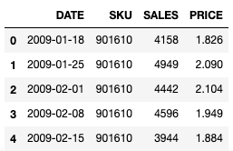
pos.head()

We have a daily timestamp of sales for many products.. We want to look at the price-demand correlation matrix for all products.
To do this, we take advantage of the pivot function in pandas. We create pivot tables of both the price and demand for all products. We can then concatenate them and call corr.
demand_matrix = pos.pivot(
    index='DATE',
    columns='SKU',
    values='DEMAND'
)

price_matrix = pos.pivot(
    index='DATE',
    columns='SKU',
    values='PRICE'
)

price_demand = pd.concat([demand_matrix, price_matrix], axis=1)
This will give us a matrix
\[\begin{pmatrix} D \,vs. D & D \,vs. P \\ P \,vs. D & P \,vs. P \end{pmatrix}\]where D is the sales (demand) and P is the price.
If we are only considering price-elasticity, then taking
rc = price_demand.shape

de_pr_corr = price_demand.iloc[0:(rc[0]/2), (rc[0]/2):column]
gives us what we want.
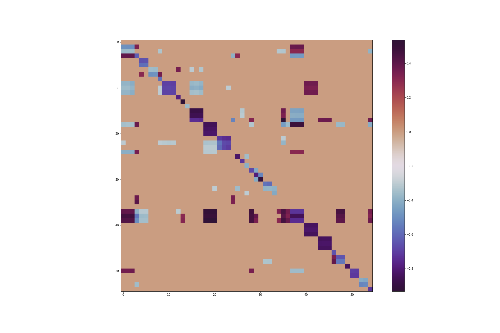
Not all products will have a strong correlation, so we elect to keep the products with strong correlations only.
Let’s visualise the relationships using a heatmap. To make it easier to identify strong correlations, we only plot correlations where $\lvert x\rvert > 0.4$.
pr_de_high_corr_only = de_pr_corr.applymap(
    lambda x: x if abs(x) > 0.4 else 0)
)

plt.imshow(pr_de_high_corr_only, cmap=plt.cm.twilight_shifted)
plt.colorbar(im)

Conclusion
Utilising price-elasticity features to model the relationship between multiple products is very common in retail.
With this correlation matrix you can identiy which products to incorporate into your analysis. You should choose only the strongly correlated products, which means that some products will have many price variables whilst others very few.
You can start by first baselining with linear regressions and incorporating price-demand variables to see how much improve there is.
Once you’re good with that, consider moving on to more complicated models, utilising time series methods (V/ARIMA) or even LSTMs.
