Optimisation is often overlooked in online machine learning courses.
Today we discuss the hello world equivalent of linear optimisation - the Simplex Algorithm.
Table of Contents
- Linear Optimisation
- What is a linear program?
- Geometric interpretation
- Basic Feasible Solutions
- The Standard Form
- Degeneracy
- Break Time
Linear Optimisation
We first construct the linear program before diving into its geometric representation and algebraic properties, all of which lead to the intuition of the algorithm. Once we understand the algorithm, we try to understand why the algorithm works mathematically.
The post assumes that you have been exposed to some 1st year linear algebra.
So what the basic form of an optimisation problem? Well, it comes in 2 parts.
The first part is an objective. Suppose you program a robot to buy as much food as possible at the supermarket. If the robot has infinite cash then it will simply buy every item in the supermarket. Hence, you also need a second part - the constraints. For example, you can tell the robot to buy only 2L of milk, not to spend more than 30 dollars on snacks and get lots and lots of vegetables =).
To formalise this, we define a set of feasible solutions $\mathcal{F}$ where each feasible solution is a possible outcome of the optimisation problem.
To determine which solution is the best one, we define an objective function (sometimes called a cost function) $c \colon \mathcal{F} \rightarrow \mathbb{R}$. In most cases we create a function that is designed so that the linear program minimises the cost.
Now let’s talk about a specific type of optimisation problem, linear programming.
What is a linear program?
A linear program (LP) is a type of optimisation problem defined by a system of linear inequalities that constrain our variables when we try to optimise for a specific objective.
Formally we define a cost function
\[\begin{align} \text{min}\left(\textbf{c}\cdot \textbf{x}\right) \end{align}\]with constraints
\[\begin{align} \textbf{A}\textbf{x}\geq \textbf{b} \end{align}\]for $\textbf{c} \in \mathbb{R}^{n}, \textbf{A} \in \mathbb{R}^{m\times n} \textbf{x}\in \mathbb{R}^{n}$ and $\textbf{b} \in \mathbb{R}^{m}$.
Here, your set of feasible solutions are $\mathcal{F} = \left\{\mathbf{x} \in \mathbb{R}^{n} \;\rvert\; \mathbf{A}\; \mathbf{x}\geq b \right\}$
Most of the time we’re going to be dealing with the linear program in standard form which is represented like below:
\[\begin{align} \text{min}\left(\textbf{c}\cdot \textbf{x}\right) \end{align}\] \[\begin{align} \textbf{A}\textbf{x} & = \textbf{b} \\ \textbf{x} & \geq 0 \end{align}\]Be very careful and don’t get confused by the 2 forms! They have algebraic properties that translate to the same geometric meaning, but the algebraic properties are not necessarily identical!
So you have a whole bunch of variables constraining your vector of $x$’s. How should we approach this?
It turns out that it is intuitively easier to understand the problem when considering the LP geometrically. This will also help shed light on the Simplex algorithm,
Geometric interpretation
Let’s look at one row of the matrix $\mathbf{A}$ at equality - $a_{i}x = b$. What does this look like in a vector space?
If $n = 1$ dimension…
\[\begin{align*} a_{1}x_{1} & = b \\ x_{1} & = \frac{b}{a_{1}} \end{align*}\]The solution to $x_{1}$ is a single point.
Now if $n = 2$ dimension…?
\[\begin{align*} a_{1}x_{1} + a_{2}x_{2} = b \\ x_{2} = \frac{b}{a_{2}} - \frac{a_{1}}{a_{2}}x_{1} \end{align*}\]And this is a straight line. In 3 dimensions the equation represents a plane.
When you generalise this to large dimensions, the equation becomes an algebraic representation of a hyperplane. When an inequality is used, the feasible vector $\mathbf{x}$’s that satisfy the inequality will lie on either side of the plane.
We call this a halfspace.
Now, since a single hyperplane can be constructed with a single row of matrix $A$ and the LP requires we satisfy the inequalities of each hyperplane, a feasible vector must lie within the intersection of all the halfspaces.
It turns out that the intersection of finite halfspaces is a polyhedron. A bounded polyhedron is always convex.
So we’ve narrowed our possible solutions to every point inside a $n$-dimensional polyhedron. Trying to solve this by brute force is not possible in a reasonable amount of time because the number of solutions will grow exponentially with respect to the number of dimensions in the vector space.
Basic Feasible Solutions
Is there a way we can narrow our search?
Well it turns out that the optimal solution can only be one of the basic feasible solutions (BFS) of the LP.
So what is a basic feasible solution? Well, a feasible solution is one inside the polyhedron. So what makes a feasible solution basic?
For a feasible solution to be basic, algebraically it must have $n$ tight constraints and the corresponding matrix $\mathbf{A}'$ formed by the $i^{\textit{th}}$ rows must be full rank.
Hang on, what is a tight constraint?
It is when the elements of $\textbf{x}$ satisfies $a_{i}x = b$, the $i^{\textit{th}}$ row of $\mathbf{A}$.
For the equation $\mathbf{A}'\mathbf{x} = \mathbf{b}'$ $\mathbf{x}$ to be the only solution, it must have $n$ tight constraints and the $\mathbf{A}’$ must be full row rank. $\mathbf{b}^{'}$ is similarly the vector of the $i^{\textit{th}}$ elements.
In other words, for a $n = 2$ dimension LP, we must have 2 tight constraints where $\mathbf{A}'\mathbf{x} = \mathbf{b}'$ hold given $\mathbf{x} = \left(x_{1}, x_{2}\right)$.
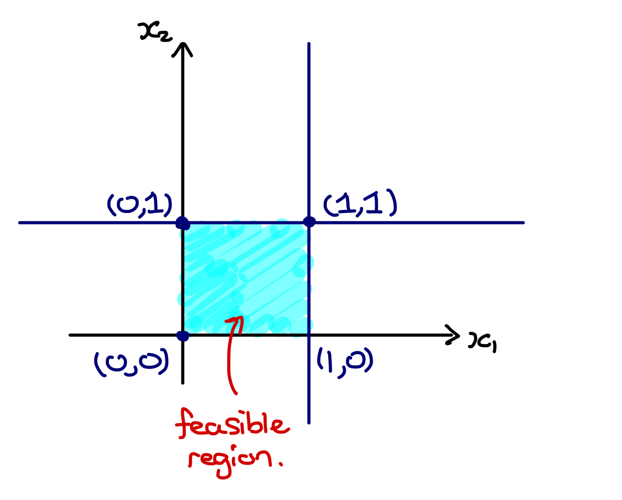
Let’s look at the example of a square. It might look something like this:

How would you describe a square using a LP?
\[\begin{align} \begin{bmatrix} - & a_{1} & - \\ - & a_{2} & - \\ - & a_{3} & - \\ - & a_{4} & - \end{bmatrix} \mathbf{x} \geq \mathbf{b} \implies \begin{bmatrix} 1 & 0 \\ -1 & 0 \\ 0 & 1 \\ 0 & -1 \\ \end{bmatrix} \begin{bmatrix} x_{1} \\ x_{2} \\ \end{bmatrix} \geq \begin{bmatrix} 0 \\ -1 \\ 0 \\ -1 \\ \end{bmatrix} \end{align}\]Take $\mathbf{x'} = [1, 0]^{T}$ for example. The 2 rows from $A$ that satisfy the equality are $a_{2}$ and $a_{3}$.
\[\begin{align} \begin{bmatrix} -1 & 0 \\ 0 & 1 \\ \end{bmatrix} \begin{bmatrix} x_{1} \\ x_{2} \end{bmatrix} & = \begin{bmatrix} -1 \\ 0 \end{bmatrix} \end{align}\]Since $n = 2$ constraints are tight, we know that this is a basic feasible solution.
Can you figure out what the other basic feasible solutions are?
When considering the LP not in standard form, we will often have more constraints than variables (this is certainly not the same with standard form LPs! I was very confused initially because I didn’t notice this).
If you have figured out the remaining basic feasible solutions, you might have noticed that they are the ‘vertices’ of the square.
This is case for all LPs - the set of basic feasible solutions correspond to the set of vertices. This is no coincidence - we can mathematically prove that the vertices and basic feasible solutions are equivalent. This is also why we talked about the geometric representation of LPs.
In other words, in order to find the optimal solution to our LP we only need to examine the vertices of the polyhedron formed by the LP.
And we need a systematic way to do that. Hence the existence of the Simplex algorithm.
Before we move onto that, we need to discuss the standard form in a little more detail.
The Standard Form
For the Simplex algorithm works with the standard form of LPs.
The important thing here to be aware of is that the standard form LP is a linear system of equations. Hence having more than $n$ equations for $n$ variables is redundant at best (when one row is a linear combination of the other rows) and can lead to an overdetermined system with no solutions.
With $m < n$ equations, we are able to fix a subset of $\textbf{x}$ variables to zero to obtain a unique solution for the remaining unfixed $\mathbf{x}$ variables. This is how we will go about finding basic feasible solutions.
The definition of a basic feasible solution remains the same, but achieving this algebraically in a standard form LP is slightly different.
We still need $n$ tight constraints for a $n$-dimensional space. However, since we have $m$ rows of equality constraints, we choose $m$ columns from $A$ such that the resulting matrix, denoted $A_{B}$, is full rank.
The set of columns we choose is defined as the feasible basis, $\mathbf{B} = \left\{b(i) \;\rvert\; i \in \mathbb{N}, 1 \leq i \leq n\right\}$, where $i$ represents the $i^{\textit{th}}$ column of $A$.
Once the columns are chosen the remaining $(n - m)$ $x_{i}$ variables, $\forall i \notin \mathbf{B}$ are set to zero.
With $m$ of the $\mathbf{x}$ variables achieving the required equality and the rest of the $n - m$ variables equal to zero (hence $x \geq 0$ achieves equality), we now have $n$ active constraints and thus our unique solution will be a basic feasible solution.
Bear in mind that a basic feasible solution and basic solution are not equivalent. If $\mathbf{x} \geq 0$ then we have a basic feasible solution. If any of the $x_{b(i)}$’s are less than zero, we have only a basic solution.
Degeneracy
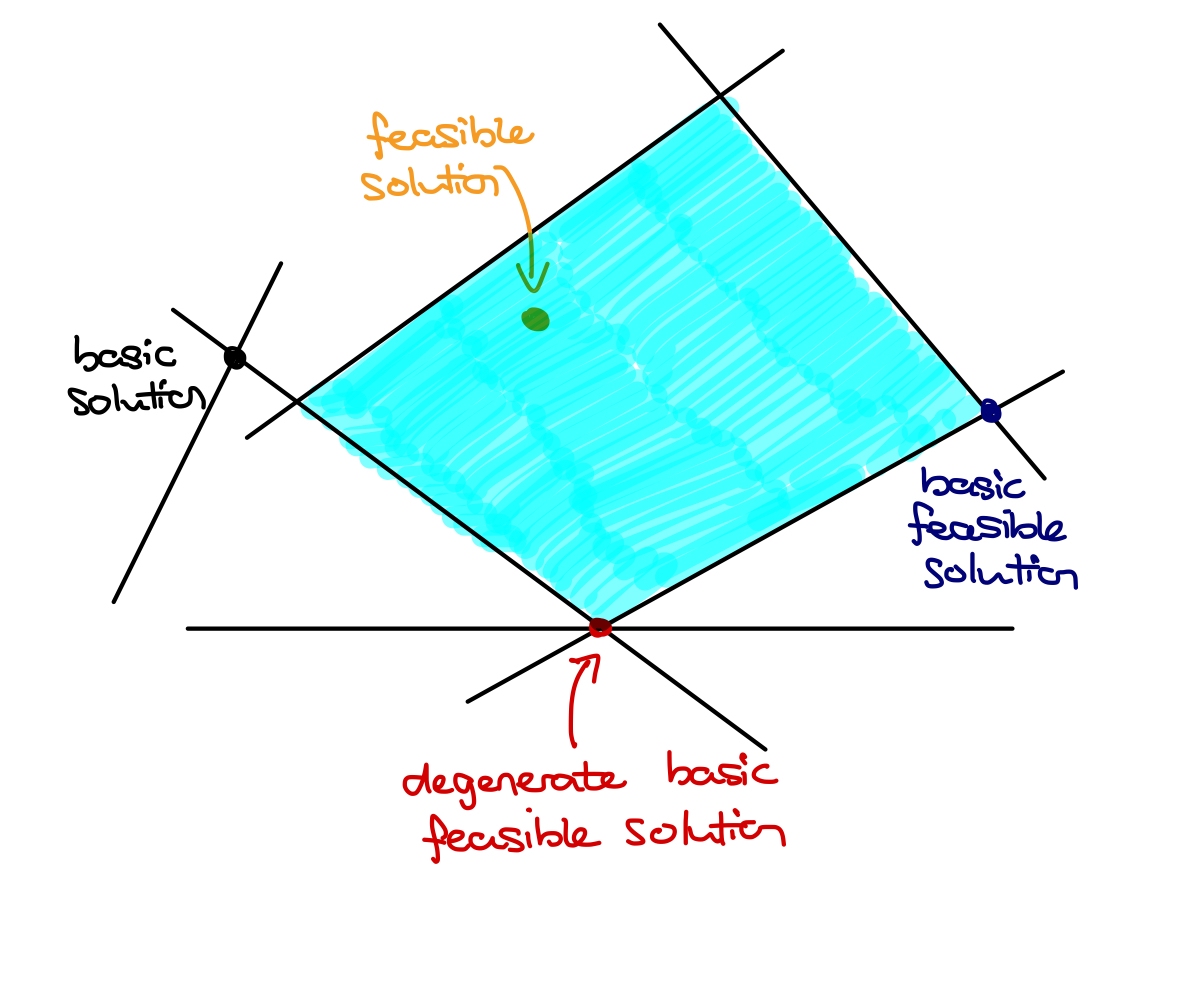
Before we talk about the mathematical definition, I want to give you a simple geometric example in words.
In a two dimension vector space, you can build a polyhedron by creating a convex hull, which when you ‘draw it out’ is just each intersection of two lines making up a single vertex (and thus a basic feasible solution).
Now, suppose for a particular vertex you also have a 3rd line passing through. In other words, you have $3 \choose 2$ possible combinations of 2 lines which intersect at the same point.
The algebraic representation of this is simple. For a given basic feasible solution, you actually have not $n$ active constraints, but more than $n$ active constraints.
For a polyhedron of standard form, you would have more then $n - m$ zero $x_{i}$’s - the unique solution $x_{B}$ given the basis matrix $A_{B}$ has at least one $x_{i} = 0$.
Here is a picture that might help:

Degeneracy is not a deal breaker, but it certainly requires us to be more careful with our Simplex implementation.
Break Time
We defined the linear problem and looked at 2 different algebraic representations of a polyhedron.
The linear program’s optimal solution must be one of the basic feasible solutions which is geometrically represented as the vertices of the polyhedron.
You can have basic and basic feasible solutions, and for each type of solution they can be degenerate or non-degenerate.
These properties come into play with considering the Simplex algorithm.
Okay, I think this is enough for one post.
Treat yourself to some coffee before the next post!
Part 2 is here
